Scalar ODE

Paper

[4] K. Jung. The specular ellipse method for scalar ordinary differential equations: exactness and accuracy up to fourth order. arXiv preprint arXiv:2608.30280, 2026.

This page reproduces the numerical experiments in the paper using specular. The six scripts save their canonical PDF figures under examples/ode/figures/.

SE2, SE3, and SE4 on this page

These labels refer to second-, third-, and fourth-order configurations of the specular ellipse method. SE2 uses sigma_n=1, SE3 uses a pointwise defect condition or a problem-specific vanishing-scale family, and strict SE4 uses the two-endpoint scale in E5a/E5b and sigma_n=1 otherwise. This SE2 is ellipse_scheme(..., sigma_n=1), which equals euler_scheme_5; it is not euler_scheme_2.

The public API also provides minimize_defect=True. That separate mode uses the full E1--E6 two-endpoint classification and may return a finite scale, the 0.0 zero-scale sentinel, or the inf Crank--Nicolson sentinel. It minimizes the classified defect but does not assert a maximal or fourth-order convergence rate. See the automatic scale-selection modes for the API and validation rules.

Install the development dependencies, then run any script from the repository root:

Copy

pip install -e ".[dev]"
python examples/ode/ellipse_exactness.py

The order statements below are numerical observations for the stated problems. The ODE guide summarizes the hypotheses required by the convergence results.

Exact tracing

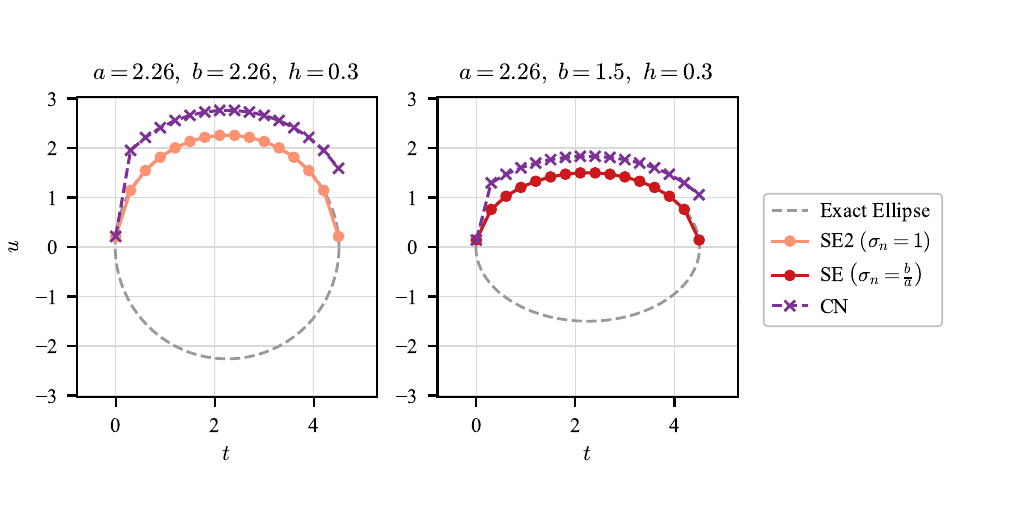
For

\[ u'=-\frac{b^2(t-p)}{a^2u}, \qquad u(t)=b\sqrt{1-\left(\frac{t-p}{a}\right)^2}, \]

the fitted scale is \(\sigma_n=b/a\). The two panels use \(p=2.25\), \(h=0.3\), and \((a,b)=(2.26,2.26)\) or \((2.26,1.5)\). The fitted SE trajectory reaches the exact ellipse at every mesh point, subject to the unique admissible implicit update assumed by the exactness result; CN does not.

Python source · PDF figure

Vanishing scales

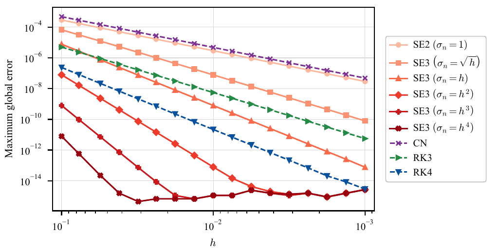
For \(u'=u^{-1}\), \(u(0)=1\), on \([0,1]\), the script compares \(\sigma_n=1\) and \(\sigma_n=h^p\) with \(p\in\{1/2,1,2,3,4\}\), together with CN, RK3, and RK4. The higher orders visible for the vanishing scales follow a direct estimate for this particular equation; they are not general SE3 guarantees. At the smallest errors, roundoff and nonlinear-solver tolerances become visible.

Python source · PDF figure

Optimal scales for a normalized pendulum branch

The normalized positive-velocity phase equation is

\[ \frac{du}{d\xi}=-\frac{\sin(\theta\xi)}{\theta u}, \qquad 0\leq\xi\leq0.8. \]

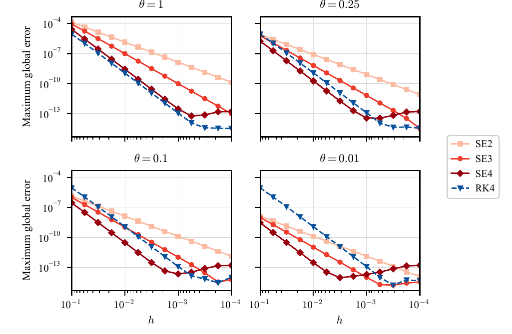
The four panels compare SE2, the pointwise SE3 selector, the two-endpoint SE4 selector, and RK4 for \(\theta=1,0.25,0.1,0.01\). This is a normalized phase equation, not the original time-domain pendulum. The curves compare accuracy at the same step size, not at the same runtime or number of field evaluations.

Python source · PDF figure

Defect cancellation for quadratic decay

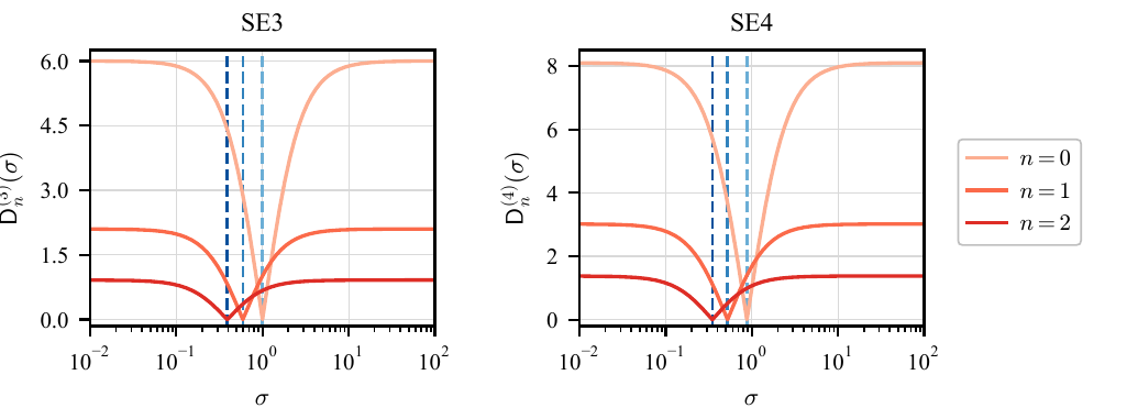
For \(u'=-u^2\), \(u(0)=1\), the two panels plot the absolute pointwise defect used by SE3 and the absolute two-endpoint defect used by SE4. The exact states at \(n=0,1,2\), with \(h=0.3\), are used so that the marked scales show the intended cancellation directly rather than accumulated global error.

Python source · PDF figure

Convergence for quadratic decay

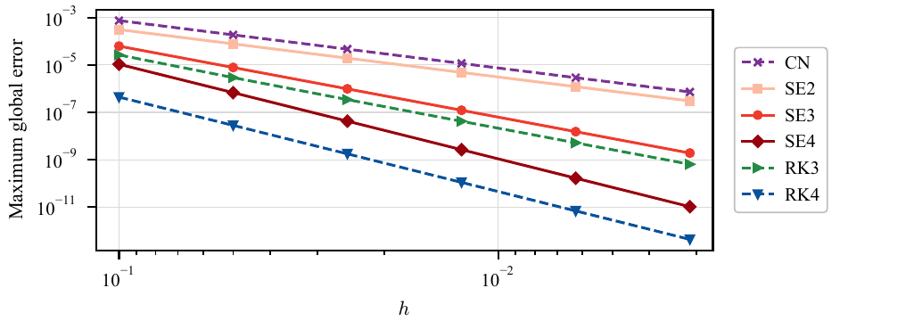
For the same quadratic decay problem on \([0,1]\), the maximum global errors show the expected second-order behavior of CN and SE2, third-order behavior of SE3 and RK3, and fourth-order behavior of SE4 and RK4. Unlike the pendulum illustration, this problem supplies a clean instance of the uniform branch assumptions used by the fourth-order convergence theorem.

Python source · PDF figure

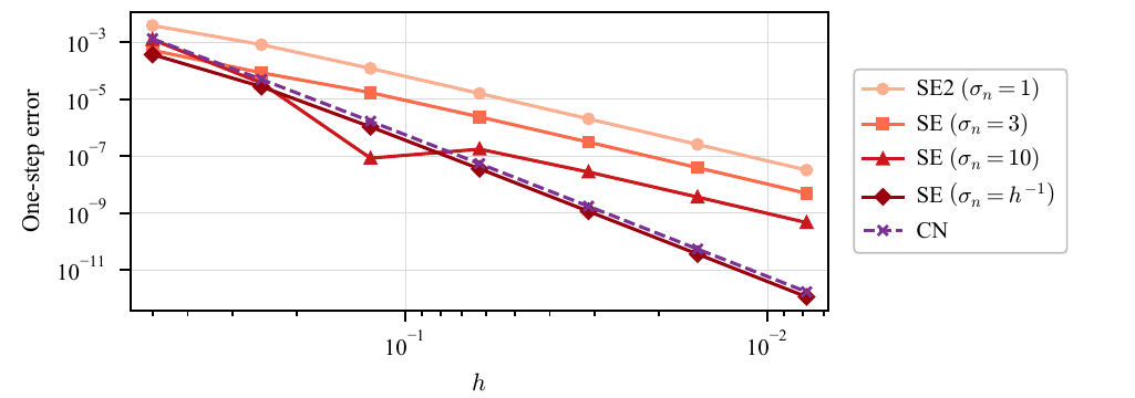
Diverging scales

For \(u'=1-u^2\), each \(h\) uses a separately selected exact endpoint pair from the large-scale boundary case. The figure compares fixed scales \(\sigma_n=1,3,10\), the diverging scale \(\sigma_n=h^{-1}\), and CN. It is a one-step experiment, not a global-convergence plot: the fixed scales exhibit third-order one-step error here, while \(h^{-1}\) and CN exhibit fifth-order one-step error.

Python source · PDF figure